Timing diagram based trace step templates¶

This section describes the use of timing diagrams as a mean to specify trace analyses. Especially the different diagram elements will be introduced by examples and the creation of timing diagrams using the diagram editor shall be explained.

The associated Reference timing diagram-based trace step templates completes this explanation with concrete annotations about the evaluation of diagrams, the basic structure and detailed definitions of all diagram elements.

Timing diagrams - introduction by using examples¶

The following figure shows a minimal timing diagram that only consists of the two always existing states precondition state and initial state. The expressions of both states are in this case signal value based. The timing diagram is activated by a transition from signal value 0 to 1. If there are no more states, signals or sample limits to interpret this timing diagram would be immediately valid. But in this example there are sample limits (1, max). The identifier max is a parameter that can be set when using this timing diagram as a trace step at the usual position. The sample limits let the state only become true if at most max times the signal value 1 appears. Otherwise the timing diagram fails because the state gets invalid. Since the sample limits of the precondition state are (0, …) the diagram is interpreted at the trace beginning (this means it is activated if the first sample of the trace has the signal value 1) as well as on every other sample of the trace.

The following timing diagram is also minimal. The precondition state has the sample limits (0, 0). In this special case the timing diagram is exclusively checked on the trace beginning. The condition is not processed and faded out for this reason. This diagram comes true if the interpreted trace starts with the timestamp 0.0 and if this only appears once. The diagram is not is not checked again.

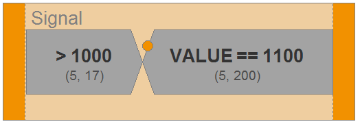
The third example shows a timing diagram that will never be activated on trace beginning because the sample limits of the precondition state (5, 17) have a minimal value greater than 0. This diagram is activated if the signal value was more than 1000 at least 5 but at most 17 times and after that a transition to 1100 takes place. This timing diagram instance is fulfilled if this signal value is repeated at least 5 but at most 200 times. If in this last state the trace end arrives or the expression of the state is evaluated to false the diagram will be true if the signal value 1100 was already found 5 times but at most 200 times.

It is possible to specify that the last state of the signal has to be valid until the end of the signal (the last sample) so it must not be left. This attribute can be set by using the context menu of the last state or the signal and by editing the signals attributes. The sample limits are still evaluated. So the signal value 1100 must occur between 5 and 200 times until the end of the signal in order to satisfy the diagram.

This is the first more complicated example, since it contains two signals with several states. If several signals are used the timelines are merged. The displayed timing diagram is activated as soon as the Signal has a transition from a signal value unequal to 0 to a signal value equal 0. With this transition occurring the second signal Signal_1 is also activated and now also those states and transitions have to be fulfilled to have the whole timing diagram come true. The next arriving real sample of Signal_1 has to match the first state expression.

An assignment is created in the initial state (marked by the star), that stores the time stamp of the current sample into the variable var. For this the key word TIME is used in the expression of the assignment. After exiting this state, the variable value is set equal to the time stamp of the last of the 8 samples with signal value 0.

This timing diagram comes true if Signal has a sample unequal to 0 followed by exactly 8 samples with a signal value of 0. Furthermore there has to be at least one more sample, whose time stamp and signal value are not evaluated in the expression. The third state checks whether the value of var that was stored in the assignment of the second state is less than 20. Aside from this also Signal_1 has to have at least three samples so that every state can be passed. First there has to be a signal value greater than 400, followed by one greater than 600, followed by one less than 1000. While evaluating, a transition from one state to another takes place as soon as possible. This means even if many signal values greater than 400 are allowed for the first state the transition is done once a signal value is also greater than 600 and the following transition as soon as a sample with a signal value less than 1000 arrives. The signal value sequence {700, 700, 700} would fulfill Signal_1 and with every sample there will be a transition to the next state because its expression is also fulfilled. The sequence {450, 500, 550, 600, 650, 700} would also fulfill Signal_1, but in this case the first state is not left before the fifth sample. As soon as the conditions of the active state and the following state do not come true the whole timing diagram will be dropped.

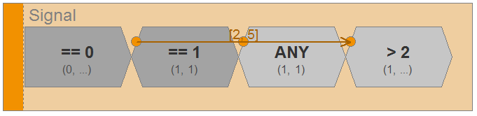
The following example shows the use of relationships. They are illustrated by an arrow from the source state to the target state. The relationship refers to the real trace time and specifies the number of time units, within which the transitions have to be done. Therefore relationships use the time stamps of the samples.

The diagram is activated by a transition from 0 to 1. It may only be one sample with the signal value 1 followed by exactly one sample of an arbitrary value (here also a 1 is possible) and within [2, 5] time units a sample must arrive with a signal value greater than 2.

Relationships can also be used between states of different signals and this shall be displayed by the extension of an earlier example. The relationship [0, 0] means that the target state has to be activated at the same time as the source state.

The samples of Signal_1 may only start with the transition to the third state of the Signal to make the timing diagram true. Now the signals are in a temporal relation to each other. Without such relationships each signal can be fulfilled individually, irrespective of whether or not initially all samples of Signal are processed and after that all samples of Signal_1 because the timelines are offset.

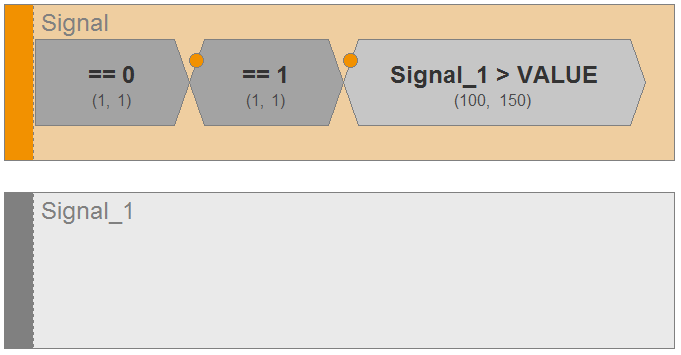
In a signal of a timing diagram the signal values of another signal can easily be accessed by using the signal name in the expression of the state. Especially signals (excluding the first signal) can be left empty if they are only used to be accessed from another signals. The following timing diagram shows such an example.

It comes true if there is a transition from 0 to 1 in Signal. After this the signal value of Signal_1 has to be greater than the signal value of Signal (represented by key word VALUE) for at least 100 and at most 150 times.

The usage of precondition states will be described by taking the following three timing diagrams as an example. For all three diagrams the activation is triggered if Signal changes from 0 to 1. The reaction of Signal_1 will be checked whether it changes from 0 to 1.

a)

Because of the precondition state ANY any values (directly before activation or after activation) of Signal_1 are accepted until value 1 is reached. The time stamp at which the second state of Signal_1 should be activated, is not specified in more detail (with activation or later).

b)

Like in case a), because of the precondition state ANY any values (directly before activation or after activation) of Signal_1 will be accepted. But by using the time constraint it is specified that Signal_1 should change to 1 not later than 0.5 after the activation of the diagram.

c)

In this case the precondition state of Signal_1 was removed. The first actual signal value after activation must match value 1. The time stamp at which exactly the second state of Signal_1 should be activated, is not specified in more detail (with activation or later.

Create timing diagrams using the diagram editor¶

Timing diagram based trace step templates are created and edited in ecu.test with the graphical diagram editor. The graphical user interface of the editor is shown in the following figure. The functions and usability concepts are described in the following chapters.

Common usability concepts¶

• Ctrl+D activates/focuses the diagram scope from anywhere.

• Ctrl+P activates/focuses the parameter table from anywhere.

• Ctrl+B activates/focuses the assignment table from anywhere.

• On confirming/saving the diagram it will be checked, if all identifiers (signal, assignment and parameter names) are unique and if not an appropriate warning is displayed.

Elements of the toolbar¶

The icons and tasks in the toolbar are from left to right:

Diagram scope¶

The diagram scope of the editor shows the currently edited timing diagram and allows the interaction possibilities that are described below.

The general handling is presented in the following table.

In normal mode (Ctrl key is not pressed) the following shortcuts and mouse activities are possible.

• Context menu (right click)

  • Free scope/timing diagram

    • add new signal (at mouse position; will be selected)

  • Signal

    • Move

    • Duplicate (directly below the selected signal; will be selected)

    • Remove

    • Add state (at the end on the selected signal; will be selected)

    • Last state must be valid until the end of the signal

  • State

    • Move

    • Remove

    • Add state (before selected state; will be selected)

    • This state must be valid until the end of the signal (if last state selected)

  • Relationship

    • Remove

In navigation mode (key Ctrl is pressed) there is no highlighting/selecting.

Panel element properties¶

The panel Element properties shows the properties of the selected element. In addtion it shows:

• the properties of all states for signals

• the properties of source and target state for relationships

The view has the following information and tasks:

• A right-click on a row opens a context menu with the options “Expand all” and “Collapse all”

• The entry of not yet existing parameter names into sample limits or time limits adds them after request

• Selection mode (no edit):

  • Up/down/right/left: choose property

  • Enter/F2: start editing (change into editing mode)

• Editing mode:

  • Enter: confirm changes (editing mode stays active)

  • Escape: cancel editing (change into selection mode)

Panel Parameters¶

The panel Parameter lists all parameters of the timing diagram and provides the following information and and functions:

• Button “+” or key “Insert” adds a parameter

• Button “x” or key “Delete” removes (the blue) parameter

• Name and type of a parameter can be edited, the name has to be unique

Panel Assignments¶

The panel Assignments lists all assignments of the timing diagram as well as of all states and relationships sorted by the corresponding elements:

• Timing diagram

• States (in the order of signals or states in signals respectively)

• Relationships (in order of adding)

The panel has the following possibilities:

• Button “+” or key “Insert” adds the assignment to the actual element (timing diagram, state, relationship)

• Button “x”or key “Delete” to delete the selected (blue) assignment

• The selection of an assignment selects the corresponding element in the editor

• The selection of an element in the diagram scope selects all associated assignments

• Name, expression and output options of an assignment can be edited

  • The name must be unique within the element

  • The expression can be arbitrarily

  • The checkbox in the column “Output” defines whether the values of the expression are forwarded outside during evaluation