Lesson 5: Signal recording and trace analysis
In this chapter, you will get to know how ecu.test evaluates time-based signal curves. This extends your test portfolio with checks that are not possible with pure test steps, for example reaction times, held states, or value ranges over time.
At the end of this lesson, your test case from Lesson 4 runs with an additional trace analysis: you record the velocity signal during stimulation and verify across the full run when a condition is fulfilled. In the Report Viewer, you see both plot and evaluation.
Prerequisites:
Lesson 4 is completed.
The
EV_Testpackage with global mapping is available.The test bench and test configuration are selected and started as described in Creating a new test bench configuration in the test bench configuration editor and test configuration editor.
Core principle of trace analysis
So far, system reactions were checked directly at runtime with read test steps. That is sufficient as long as single values at specific points in time are relevant.
In many real-world use cases, however, temporal behavior matters: does a signal react within a defined time after an input changes? Is a state held for a certain phase? Does a signal stay inside a valid range throughout the test? Such time-based checks are better performed after stimulation, using trace analysis.
During test execution, signal curves are recorded. This recording is then evaluated by the trace analysis. The results are shown in a dedicated section of the test report, including both condition results and graphical views of the evaluated signals. This allows us to draw conclusions about reaction times, ranges of values, temporal sequences, and the interaction of multiple signals.
Trace analysis extends the test to include an evaluation of temporal relationships between signals.
Example: Temporal relationships between signals
Whenever the green signal reaches value 1, then the red signal has to take value 1
within 1 ms and retain this value for at least 5 ms.

Info
In ecu.test, stimulation and evaluation are separated. The test case stimulates the system, and trace analysis evaluates the recorded signals afterwards. This allows you to reuse the same stimulation with different evaluations without changing the test case.
Components of a trace analysis
- Signal recording
Defines which signals are logged during test execution.
- Plot
Visualizes the recorded signals.
- Trace analysis
Formulates and checks conditions on recorded signals.
- Report entry
Shows plots and condition results in the Report Viewer.
Add a trace analysis to an existing test case
Let us extend the test case from Lesson 4 by adding trace analysis. To do this, you enable signal recordings, create a Trace analysis with plot and condition, and execute the test case.
Create a trace analysis
A dedicated trace analysis area is created in the package. It is initially empty.
Open the
EV_Test.pkgpackage from Lesson 4 in the test case editor.Switch to the Trace Analysis tab.
Create a new trace analysis using the add button.
Enter a name and confirm with OK.
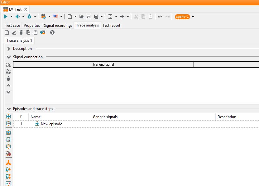
A newly added and initially empty trace analysis.
Define a condition
You define a time-based condition for velocity from the global mapping (Lesson 4): the check validates that the speed is greater than 50 km/h.
Open the loaded global mapping in the mapping file editor.
Right-click velocity and add a calculation to the trace analysis for this variable.
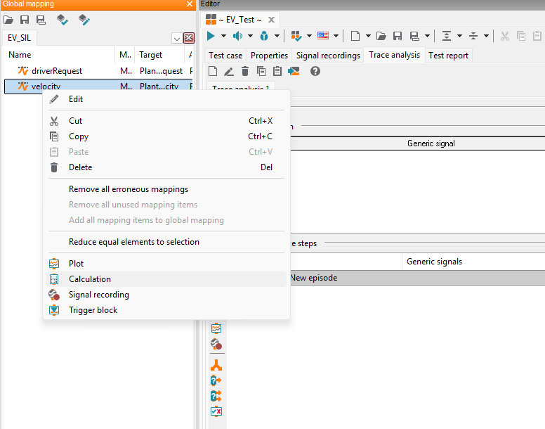
Double-click the newly added calculation step.
Add
> 50to the expression.Confirm with OK.
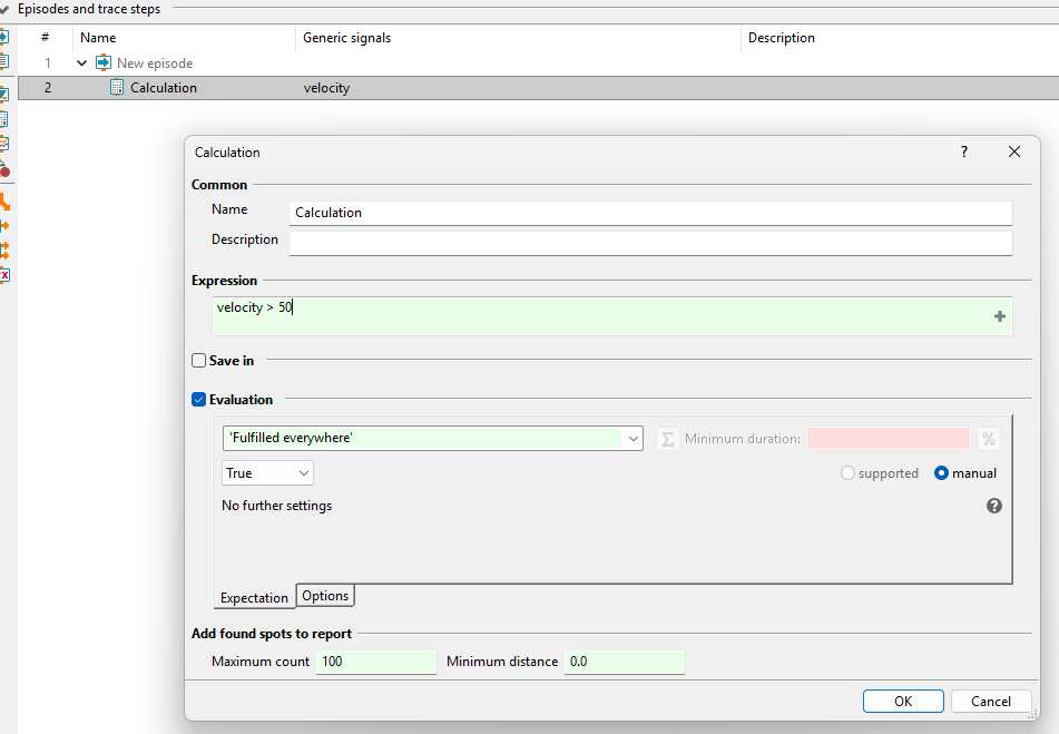
This creates a condition that checks whether velocity > 50 is fulfilled.
Add a plot
To display the signal curve graphically, add a plot and assign it to the condition.
Right-click velocity again in the global mapping and select Add Plot.
Drag and drop the plot into the calculation step.
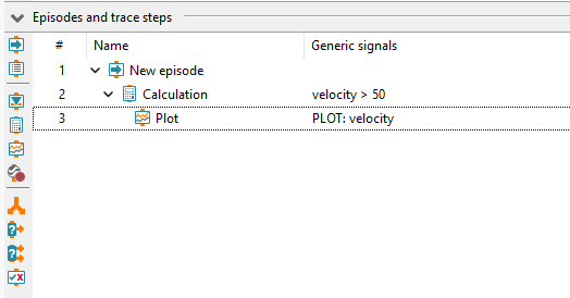
The plot is now linked to the condition and appears in the report together with the condition result.
Configure a signal recording
For trace analysis to evaluate data, velocity must be recorded during the test case.
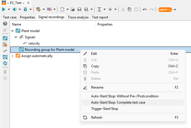
Switch to the Signal Recording tab.
Add a signal recording in the package for the model access.
Right-click the signal recording group.
Select Automatic Start/Stop: Complete test case.
Save the package with Ctrl+S.
Info
Instead of variables from the global mapping, you can also use variables from model access or other domains. They are selected in the same way: via the context menu or by dragging and dropping them into the trace analysis window.
Execute a test case and verify the trace analysis in the report
Press F9 or click Run test case in the package editor.
After execution, open trace analysis under Analysis Jobs in the Test Report tab.
Check the signal plot and the condition result below the plot.
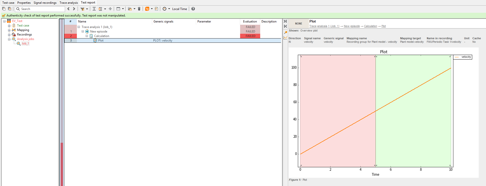
The report shows the velocity curve and the evaluation for > 50. Because the vehicle
is stationary at the start of the test case, the condition is initially not fulfilled. After a few
seconds, the status changes to fulfilled.
Result of lesson 5
In this lesson, you extended the Lesson 4 test case with trace analysis: the velocity signal is recorded over the complete test case, linked to a condition, and reported as a plot with evaluation. This is your first check evaluated over time instead of at a single point.
Even a simple trace analysis with one plot and one condition provides significantly more insight than pure read test steps. Separating stimulation and evaluation also allows both to be maintained and combined independently.
Further topics related to Trace analysis are described in detail in the following sections: